* ACCESS THE FOLLOWING LINKS (ALL ON THIS WEBSITE) OR DROPDOWN MENU ABOVE FOR CURRENT RECOMMENDED ATMOSPHERIC CORRECTION AND SURFACE REFLECTANCE GUIDES FOR LANDSAT 8 & SENTINEL-2; GUIDES ARE DESIGNED FOR ARCGIS OR FREE QGIS. *
2022 Landsat 9 & 8 Conversion to Surface Reflectance (different than prior years)
Landsat 8 w/ArcGIS • Landsat 8 w/Free QGIS • Sentinel-2 w/ArcGIS • Sentinel-2 w/ Free QGIS
For Less Detail Use: Simplified Landsat 8 & Sentinel-2 Conversion to Surface Reflectance Steps
Click Here for a List of Atmospheric Correction Background Links on this Website
_____________________________________________________________
Landsat 8 Atmospheric Correction Guide
Includes COST, DOS, and TOA reflectance
(Lowest Valid Value, Preferred Method [continuous relative scatter], and Dark Object haze removal)
 (NASA, 2013)
Landsat 8 COST vs. DOS Surface Reflectance
The COST model (Chavez, 1996) has been shown to be more accurate than the DOS (Chavez, 1988) or TOA models for Landsats 5 and 7 due to the inclusion of an additional cosine factor in the denominator (Chavez, 1996). However, Landsat 8 has many differences compared to previous Landsats including a much different (and improved) NIR bandwidth. ESUN values were established for Landsat 8 in order to determine if the COST or DOS method should be used to calculate surface reflectance (TOA is not surface reflectance). Important: The COST model was tested and developed, as well as compared to the DOS model, mainly under the parameters of: 1) visible band reflectance being < 0.2; 2) near infrared (NIR) reflectance being > 0.2; and 3) the solar elevation being ≥ 45° - it should not be assumed that the accuracy of retrieved reflectance from either the DOS or COST model based on values outside these parameters is the same as the accuracy of retrieved reflectance based on values within the parameters when applied to any Landsat satellite imagery, including Landsat 8 as described by GIS Ag Maps.
Correct ESUN values were calculated by GIS Ag Maps and are listed and described in the Landsat 8 ESUN Values section of the Landsat 8 ESUN, Radiance, and TOA Reflectance page. A comparison was made here between Landsat 8 COST and DOS with the objective of providing information to help determine the better atmospheric correction model for Landsat 8. To GIS Ag Maps knowledge, this is the first Landsat 8 reflectance comparison made between the different reflectance models. It is important to understand that more research needs to be done to make a general conclusion about whether COST or DOS should be used for Landsat 8. The research here corresponds to a particular surface and condition; a conclusion as to whether COST or DOS is better for Landsat 8 should be based on research that encompasses more surfaces and conditions such as the Chavez (1996) research did that showed COST was a superior method. The research and information from GIS Ag Maps supports DOS as the better overall method for Landsat 8 surface reflectance mainly due to more accurate NIR reflectance values. Landsat 8 DOS versus COST reflectance results follow: Landsat 8 DOS vs. COST NIR Reflectance Landsat 8 vs. Landsat 7 LEDAPS Field Reflectance Landsat 8 vs. Landsat 7 LEDAPS Reflectance.
Landsat 8 DOS and COST Methods
(easier conversion to surface reflectance)
Whether using DOS or COST for Landsat 8, steps necessary in the atmospheric correction process can be reduced compare to previous Landsats because terms have been embedded in Landsat 8 DN values. Simply apply the steps in the following paragraph to convert to Landsat 8 DOS or COST Method surface reflectance (Landsat 8 DOS Method and Landsat 8 COST Method were published by GIS Ag Maps at www.gisagmaps.com on 9/5/2013 and are based on the DOS method from Chavez [1988] and COST method from Chavez [1996]).
To calculate Landsat 8 DOS or COST Method surface reflectance:
1) Apply the following equation to the entire raster for each band: ([DN x .00002] - 0.1).
2) Divide the values from Step 1 by the cosine of the solar zenith if calculating DOS reflectance or the (cosine of the solar zenith)² for COST reflectance. The solar zenith = (90 - solar elevation); the solar elevation given in the .MTL file can be used or a more local value can be used if available.
3) Establish the scatter DN (there are different methods for this as is explained in the tutorial and below; the Lowest Valid Value from band 4 [red] in conjunction with the Continuous Relative Scatter Lookup Table is the recommended method here and is described in the Preferred Method example in the tutorial). If not applying relative scatter, the Lowest Valid Value for individual bands can be used. (the Lowest Valid is value is the lowest value that is more than any break of values ≥ 100 in the low end of the histogram, which may not be the very lowest value).
4) Apply the following equation to the scatter DN from Step 4: ([DN x .00002] - 0.1).
5) Divide the scatter value from Step 4 by the cosine of the solar zenith if calculating DOS reflectance or the (cosine of the solar zenith)² for COST reflectance (as explained in Step2).
6) This is an optional step. THE CURRENT PREFERRED METHOD DOES NOT APPLY ONE-PERCENT REFLECTANCE. WHILE IT IS NECESSARY TO CONVERT VISIBLE BANDS TO SURFACE REFLECTANCE, TOA REFLECTANCE SHOULD BE USED FOR BANDS 5 & 6 (AS IS SHOWN IN THE PAGE) IF THE GOAL IS TO DERIVE SURFACE REFLECTANCE MORE SIMILAR TO USGS LANDSAT 8 SURFACE REFLECTANCE.
Though deducting .01 from haze (in order to acquire one-percent reflectance from the established low value) has been shown to improve accuracy when applied to previous Landsats, analysis here based on the Lowest Valid Value from the Landsat 8 attribute table shows that IF THE GOAL IS TO RETRIEVE REFLECTANCE MORE SIMILAR TO USGS LANDSAT 8 SURFACE REFLECTANCE, IT IS BETTER TO BYPASS (NOT APPLY) THIS STEP BASED ON RESEARCH HERE and simply deduct scatter (haze) from the different bands based on the relative scatter table. This could be due to a variety of reasons. Check back or contact GIS Ag Maps for more information and analysis. Chavez (1996) deducted .01 from the established scatter reflectance so the dark object has one percent reflectance (which is .01 in reflectance units) as "one percent minimum reflectance is better than zero percent".
7) Subtract the scatter reflectance values from corresponding band reflectances derived from Step 2 to derive DOS or COST surface reflectance. This is much simpler than the standard conversion to reflectance method (results may vary at the 100,000 place based on ESUN values listed in website).
Using dark objects (explained below) to base scatter on will produce similar values than if basing scatter on the Lowest Valid Value Method (explained below) for each band individually. The preferred method is outlined next and is described in more detail in the Landsat 8 Reflectance Tutorial.
* Preferred Method of Landsat 8 Atmospheric Correction *
The Preferred Method to convert Landsat 8 to surface reflectance combines the above Landsat 8 DOS Method with the Continuous Relative Scatter Lookup Table (based on a starting scatter value from band 4 [red]); the method is explained and can be calculated through the Landsat 8 Reflectance Tutorial. The best way to understand the Preferred Method is to access the Landsat 8 Reflectance Tutorial, download the data, and follow the steps in the Preferred Method section to calculate reflectance. However, Landsat 8 Preferred Method reflectance can be acquired already calculated as File 4 from the LEDAPS Reflectance & Index Downloads page (includes the values and steps used for reflectance calculation).
Landsat 8 Traditional Method Atmospheric Correction Guide
The information below describes how to convert Landsat 8 imagery to reflectance based on COST (Chavez, 1996), DOS (Chavez, 1988), and TOA models.
Related pages: Atmospheric Correction (more details) Landsat 8 ESUN, Radiance, and TOA Reflectance
DOS better than COST for Landsat 8 (COST is necessary for previous Landsats): NIR Comparison Visible, NIR, and SWIR Comparison
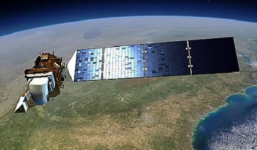
This guide describes how to convert Landsat 8 data to reflectance through atmospheric correction. Reflectance is the ratio of total radiation reflected off a surface to the total incoming radiation. Landsat imagery is free and has near world-wide coverage. Reflectance enables imagery to be applied in many more ways.
The cosine of the solar zenith angle correction (COST) model (Chavez, 1996; pdf, opens in new tab) can be written as:
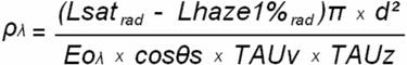
(For COST: "CO" is from cosine; "S" is from solar; the "T" is from "TAUz". Eoλ is also referred to as ESUN; TAUv = 1.0 for Landsat; TAUz = cosθs for COST method.)
It is important to keep in mind that the COST method has not be studied for Landsat 8, which has different bandwidths than previous Landsats. The method has been shown to improve reflectance accuracy for certain surfaces compared to the TOA and DOS methods (listed below) for previous Landsats, but may or may not be the most accurate for Landsat 8.
The COST model is described in detail in the Atmospheric Correction Guide page and in the Landsat 5 & 7 Tutorial in the top drop-down menu: it will be applied step-by-step here to explain how to convert Landsat 8 to reflectance.
The dark-object subtraction (DOS) model (Chavez, 1988) is the above COST model with TAUz omitted.
The top of atmosphere (TOA) model (also known as apparent reflectance or in-band planetary albedo) is the above COST model with the deduction for scatter and TAUz omitted.
Step 1: Lsatrad
Lsatrad is the radiance at the satellite sensor. Landsat imagery pixel values are in digital number (DN) format. DNs represent calibrated amounts based on radiance. The DNs need to be convert back to radiance; this is done through an equation based on values n the .MTL file that is included with the imagery upon download. The following is from the USGS (2013) and shows how to convert DNs to radiance for Lansat 8:
OLI and TIRS band data can be converted to TOA spectral radiance using the radiance rescaling factors provided in the metadata file:
Lλ = MLQcal + AL
where:
Lλ = TOA spectral radiance (Watts/( m2 * srad * μm))
ML = Band-specific multiplicative rescaling factor from the metadata (RADIANCE_MULT_BAND_x, where x is the band number)
AL = Band-specific additive rescaling factor from the metadata (RADIANCE_ADD_BAND_x, where x is the band number)
Qcal = Quantized and calibrated standard product pixel values (DN)
Step 2: Lhaze1%rad
Lhaze1%rad is the most time-consuming component of the equation. This represents the amount radiance is incorrectly increased at the sensor due to the effect of atmospheric haze (this amount is also known as path radiance or scatter); haze radiance needs to be deducted from total radiance of applicable bands. As solar radiation travels through space and enters Earth's atmosphere it can strike particles in the atmosphere and reflect back to the satellite sensor, erroneously increasing radiance values. The theory behind image-based correcting for the effect of haze is that within a Landsat scene (which contains millions of pixels) there should be a surface that reflects no radiation; the amount this surface is above zero reflectance is to due to haze. However, because of " the fact that very few targets on the Earth's surface are absolute black...an assumed one-percent minimum reflectance is better than zero percent" (Chavez, 1996). Subtracting .01 reflectance units from the haze reflectance will result in the established haze (dark object) as having one-percent reflectance. Establishing the haze amount will be detailed later in this section. There are different methods to establish a haze amount; it is not a rule to use the very lowest pixel value.
Calculating Lhaze (1%rad will be described after)
There are different ways to calculate the effect of haze. Methods that applied to Landsat 4, 5, and 7 do not necessary apply to Landsat 8. Methods here include Relative Scatter (values are listed in the Landsat 8 Haze Removal & Lookup Table page), Lowest Valid Value, and Dark Object. Reflectance values based on the different haze removal methods are included near end of page.
Continuous Relative Scatter vs. Lowest Valid Value
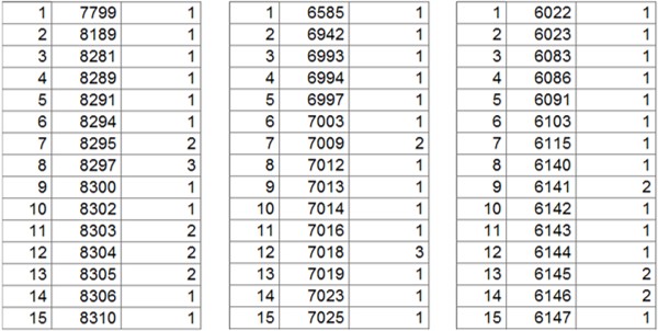
Continuous Relative scatter can be applied based on a starting scatter reflectance value (using the Landsat 8 DOS or Cost Method to calculate surface reflectance); the corresponding bands can then have relative scatter applied (based on scientific principles and past research). Relative scatter values are listed and the method is described in the Landsat 8 Haze Removal & Lookup Table. If applying continuous relative scatter, convert the green band to one-percent reflectance based on the lowest valid value, then select corresponding relative reflectance from the Continuous Haze Look-Up Table (can be accessed through the previous link). If applying the Lowest Valid Value method, it is not a rule that the lowest pixel value in the histogram should be selected as the haze amount. A method to establish a DN scatter amount can be to use the lowest DN that is more than any break of values ≥ 100 in the low end of the histogram. Based on a typical solar zenith cosine value, a break of 100 corresponds to approximately .0025 reflectance units (a quarter percent); it is more likely that a DN value associated with a break such as this is affected by something nonphysical and is erroneous than a DN not associated with such a separation. A break of over 900 is shown in a histogram example in the Haze Removal and Lookup Table page. If using this method for the data below, values would be 8189, 6942, and 6022 for the blue, green, and red bands, respectively. A Landsat 8 NIR scene commonly has many DN values that correspond to negative reflectance. Of the twenty-three images assessed here, four have had any value at all above zero reflectance; none of those four have been greater than .01 reflectance which is a realistic minimum reflectance.
Landsat 8 histogram values for, from left to right: band 2 (blue); band 3 (green); band 4 (red)
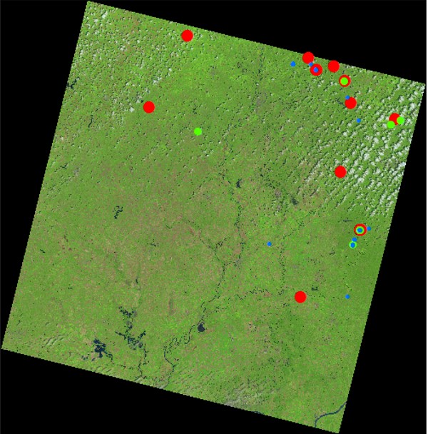
Dark Object Selection Method
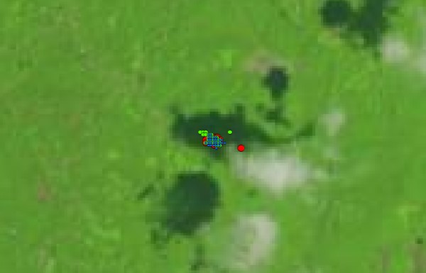
Haze can be based on a true visible band dark object area or pixel. See more dark object examples here. Dark object-based haze will result in similar values as the Lowest Valid Value method described above. For Landsat 8 haze selection here, a dark object corresponds to an area of vegetation in cloud cover where there are very relatively low values in the red, green, and blue bands (center-right); the dots are centered on pixels where the colors represent the corresponding red, green and blue bands. The dark object method typically produces values that are very similar to the lowest valid value method described above.
Zoomed in to dark object area you can see there are many low values and that they correspond to a shadow in an area of vegetation.
The low value pixel area can be viewed with higher resolution imagery below (the LandsatLook imagery above is based on Landsat 30 x 30 meter pixels). The low value pixels above correspond to the center area of the image below (extent of the images are similar but not exactly the same). It can be seen by viewing both images that the low values in the visible bands at the time of imaging correspond to green vegetation which is a high absorber of visible radiation (green vegetation reflects more green light than blue and red, but green reflectance is still low). The already low visible band reflectance amounts are lowered by the shadows from clouds, and possibly from trees and/or topography. For these reasons, it makes sense that this is an area of minimal visible light reflectance. NIR reflectance may not be the lowest here because of the associated vegetation; NIR can transmit through shadows and reflect the surface.
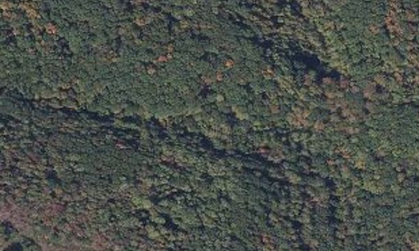
(Bing imagery)
From the cluster of points in the dark object area above, the lowest DN in each band should be selected as the haze value (unless there is an obvious erroneous value) and converted to radiance (lowest values do not need to be from the same pixel but in the same dark object area). There should be a power relationship between band haze (path) radiance (Chavez, 1988). Longer wavelength will have relatively less haze. Clearer atmospheres will have a greater path radiance difference between bands. Hazier atmospheres will have more path radiance for all bands and the haze amounts will be more similar between bands. The haze radiance below shows that a strong power relationship exists. Haze deduction does not have to be applied to bands longer that NIR.
The following are the haze radiance values before the one-percent reduction as detailed in the Landsat 8 Atmospheric Correction page:
Band Band Center Haze DN Haze Radiance
2 (blue) .480 8289 41.876908
3 (green) .560 6993 23.234554
4 (red) .655 6140 11.255974
The band center and haze radiance values from above are plotted below with a power line.
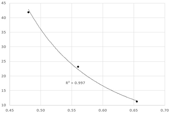
If it is difficult to find pixels in dark object areas with your software, keep in mind that the values shown below (in the tables after the next paragraph) are very low. If you prefer, to establish haze amounts simply fit low radiance values from the blue, green, and red bands (as well as the NIR band, if applicable, as is described in the main Atmospheric Correction Guide page) to a power line with a high correlation, avoiding low values that have a large gap between them and the rest of the data (as the lowest values in the blue and green data below). This gap can commonly exist somewhere at the very low end of the histogram, it does not always exist between the lowest value and the rest of the data, but could be between a very low value and the rest of the data. Because values are low, make sure that the DNs you select for different band haze amounts correspond to radiances greater than zero; there may be some digital number near the low end of the histogram that correspond to negative radiance values. Negative radiance mainly applies to the NIR band however; is it unlikely for visible bands.
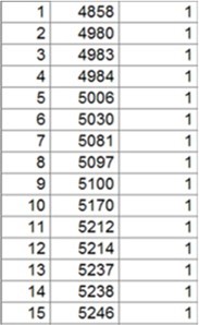
Landsat 8 low end of histogram data that show selected haze DNs; from left to right DNs are, band 2 (blue), 8289; band 3 (green), 6993; and band 4 (red), 6140. Landsat 8 data is based on a 12-bit dynamic range but are delivered as 16-bit images; previous Landsats were based on 8-bit for both. Landsat 8 DNs have a maximum value of 65,535 as opposed to previous Landsat which had a maximum value of 255. The number in the left column of each table is the ranking of the DN value (1 is the lowest DN in the entire scene); the number in the middle column is the DN value; and the number in the right column is the amount of the DN values there are in the entire scene.
If the histogram for band 5 (NIR) shows DN values that correspond to zero or negative radiance (there can be times where NIR or larger bands have some pixels that correspond to zero or negative radiance) such as it does in this example (5000 equals zero radiance), there is no need for haze deduction. Sometimes NIR should have a haze deduction and sometimes it should not. There is an example where NIR haze should be deducted in the Atmospheric Correction Guide.
Band 5 low end of histogram (5000 equals zero radiance)
As previously mentioned, bandwidths longer than NIR (such SWIR) do not need haze deducted.
Calculating 1%rad to deduct from Lhaze
Once the haze (path) radiance has been calculated, one percent should be deducted from that amount because of " the fact that very few targets on the Earth's surface are absolute black, so an assumed one-percent minimum reflectance is better than zero percent" (Chavez, 1996).
The following equation should be used to calculate one-percent reflectance for each band individually and the amount should be deducted from the haze radiance of each band, that way when the one-percent radiance amount is subtracted from the haze radiance, the resulting amount will be one-percent reflectance instead of zero. (The value derived by the following equation when input into the atmospheric correction equation will derived .01 reflectance; or for COST model, [value x pi x d²] / [Eoλ x cosθs²] = .01; for DOS model, [value x pi x d²] / [Eoλ x cosθs] = .01)
One percent reflectance equation (ARSC, 2002) equals one percent of the denominator of the COST equation above, which = 0.01 x ([Eoλ x cosθs²] / [d² x pi]); for DOS model, TAUz is omitted in atmospheric correction process, then equation = 0.01 x ([Eoλ x cosθs] / [d² x pi]).
Eoλ (also referred to as ESUNλ)
Landsat 8 ESUNλ values have not been made publicly available; however, they have been derived by GIS Ag Maps. The Landsat 8 ESUN, Radiance, & TOA Reflectance page describes in detail how the derived ESUN values were calculated; it is important to view the page to understand the basis of the values. The derived ESUN values are as follows:
| Landsat 8 | ESUN | ||||||
| Band | TOA * | ||||||
| 2 | 2067 | ||||||
| 3 | 1893 | ||||||
| 4 | 1603 | ||||||
| 5 | 972.6 | ||||||
| 6 | 245.0 | ||||||
| 7 | 79.72 | ||||||
| 9 | 399.7 |
Band 1 is indigo and is used for coastal applications; Band 8 is panchromatic; bands 10 and 11 are thermal and can be converted to at-satellite brightness temperature as shown near the bottom of this page.
ESUN TOA* The ESUN value are derived by solving for them in the standard TOA equation (for a single scene); where, TOA reflectance = ([at sensor radiance] x pi x [earth-sun distance²]) / (cosine of solar azimuth) x ESUN. Landsat 8 TOA reflectance can be computed per USGS (2013) as shown near the bottom of this page (the sun angle factor should be applied for TOA reflectance as mentioned by the USGS when describing their TOA equation). When the ESUN TOA values above are input into the standard TOA reflectance equation, the calculated reflectance is the same (to four significant figures) as the value calculated by the USGS Landsat 8 TOA equation.
cosθs²
This is the cosine of the solar azimuth. The solar azimuth = (90⁰ - solar elevation). The solar elevation is listed in the .MTL file that is included with the Landsat imagery upon download. A single cosine value is commonly used for any area in the entire image. However, you may find tools on-line to derive local values. Chavez (1996) determined that cosθs could be used for TAUz (which accounts for atmospheric transmittance along the path from the sun to the ground surface).
d²
This (d) is the Earth-sun distance and is included in the .MTL file. The d value needs to be squared.
Π (pi)
The value of pi = 3.14159265
At this point, all the variables of the 1% percent reflectance equation applied to the COST model have been described. Once again the equation is,
1% reflectance = 0.01 x ([Eoλ x cosθs²] / [d² x pi])
When the value derived by the 1% reflectance equation is input as the parenthesis value in the numerator in the COST equation (shown below), and the the equation is calculated (the 1% value is multiplied by pi and d²) the resulting value will be .01.
At this point Lhaze1%rad can be calculated by determining the haze value for each band (not necessary for bands larger than NIR), converting the DN value to radiance by the method shown in Step 1, and subtracting the 1% reflectance value from the haze radiance.
Step 3: Calculate Reflectance Based on the COST, DOS, and Models
By viewing the COST equation below and the information in Steps 1 and 2, you will notice that all the components of the COST equation are accounted for.
(Eoλ is also referred to as ESUN; TAUv = 1.0 for Landsat; TAUz = cosθs for COST method)
The dark-object subtraction (DOS) model (Chavez, 1988) is the above COST model with TAUz omitted.
The top of atmosphere (TOA) model (also known as apparent reflectance or in-band planetary albedo) is the above COST model with the deduction for scatter and TAUz omitted.
You can now calculate reflectance by using a raster calculator in GIS software. Reflectance has many more applications than DNs, such as calculating NIR reflectance or indices to assess vegetation condition or to input reflectance-based values in models to assess condition and predict yield. Mean reflectance values for bands 2 - 6 for this atmospheric correction for the imagery shown in the Landsat 8 Color and Band Graphics page follow (LandsatLook natural color image for data is shown below). Although there was a mixture of surfaces, most was vegetation; as a result, there is much higher NIR reflectance than visible band reflectance. COST and DOS green (band 2) has higher reflectance than blue or red due to the vegetation; TOA does not represent surface reflectance and, a result, has higher blue reflectance than green.
The below values have been updated to show reflectance values that result from entering precisely the same values from the tutorial (same amount of values after decimal point). If your results are different when calculating with raster calculator, take the mean of the DN raster (in Quantum GIS, you can right-click on raster layer, then click Properties then Metadata to find mean values) and input it into an Excel spreadsheet (or other spreadsheet) to check raster calculator results.
Mean (based on Relative Scatter path radiance)
| COST | DOS | TOA | |||||
| Band 2 | 0.055 | 0.051 | 0.110 | ||||
| Band 3 | 0.073 | 0.067 | 0.100 | ||||
| Band 4 | 0.062 | 0.057 | 0.073 | ||||
| Band 5 | 0.455 | 0.414 * | 0.414 * | ||||
| Band 6 | 0.226 | 0.205 * | 0.205 * |
Mean (based on Lowest Valid Value path radiance)
| COST | DOS | TOA | |||||
| Band 2 | 0.052 | 0.048 | 0.110 | ||||
| Band 3 | 0.073 | 0.067 | 0.100 | ||||
| Band 4 | 0.066 | 0.061 | 0.073 | ||||
| Band 5 | 0.455 | 0.414 * | 0.414 * | ||||
| Band 6 | 0.226 | 0.205 * | 0.205 * |
Mean (based on Dark Object path radiance)
| COST | DOS | TOA | |||||
| Band 2 | 0.052 | 0.048 | 0.110 | ||||
| Band 3 | 0.072 | 0.066 | 0.100 | ||||
| Band 4 | 0.063 | 0.058 | 0.073 | ||||
| Band 5 | 0.455 | 0.414 * | 0.414 * | ||||
| Band 6 | 0.226 | 0.205 * | 0.205 * |
* Bands 5 (NIR) and 6 (SWIR) did not have a haze deduction as explained in the tutorial (NIR sometimes does; haze deduction is not necessary for SWIR), so the DOS and standard TOA reflectance equations are the same. TOA reflectance was calculated with the standard TOA equation instead of the USGS Landsat 8 equation (shown below). The Landsat 8 TOA equation may derive very slightly different reflectance than the standard TOA equation (values at the 10,000th place may be slightly different).
LandsatLook natural color image extent for data represented by above statistics

Landsat 8 Equations to Convert to Radiance, TOA Reflectance, and At-Satellite Brightness Temperature (USGS, 2013b)
Conversion to TOA Radiance
OLI and TIRS band data can be converted to TOA spectral radiance using the radiance rescaling factors provided in the metadata file:
Lλ = MLQcal + AL
where:
Lλ = TOA spectral radiance (Watts/( m2 * srad * μm))
ML = Band-specific multiplicative rescaling factor from the metadata (RADIANCE_MULT_BAND_x, where x is the band number)
AL = Band-specific additive rescaling factor from the metadata (RADIANCE_ADD_BAND_x, where x is the band number)
Qcal = Quantized and calibrated standard product pixel values (DN)
Conversion to TOA Reflectance
OLI band data can also be converted to TOA planetary reflectance using reflectance rescaling coefficients provided in the product metadata file (MTL file). The following equation is used to convert DN values to TOA reflectance for OLI data as follows:
ρλ' = MρQcal + Aρ
where:
ρλ' = TOA planetary reflectance, without correction for solar angle. Note that ρλ' does not contain a correction for the sun angle.
Mρ = Band-specific multiplicative rescaling factor from the metadata (REFLECTANCE_MULT_BAND_x, where x is the band number)
Aρ = Band-specific additive rescaling factor from the metadata (REFLECTANCE_ADD_BAND_x, where x is the band number)
Qcal = Quantized and calibrated standard product pixel values (DN)
TOA reflectance with a correction for the sun angle is then:
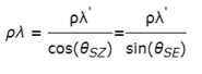
where:
ρλ